Tutorial: Analysis with Starlink

Worked Example

The first file we are going to look at is an archival HARP map jcmth20061220_00044_01_reduced001_nit_000.fits

This is a 2006 reduced cube containing a CO 3-2 HARP observation of Ros 6.

The first thing we will do is convert it from FITS format into NDF — the Starlink data format. To do this we need to inialise the convert package:

$convert
CONVERT commands are now available -- (Version 1.8)
 
 Defaults for automatic NDF conversion are set.
 
 Type conhelp for help on CONVERT commands.
 Type "showme sun55" to browse the hypertext documentation.

We then run the command fits2ndf:

$fits2ndf jcmth20061220_00044_01_reduced001_nit_000.fits co32_cube.sdf

JCMT archive data uses Barycentric Frequency as its frequency coordinate system; use ndftrace to examine this. First of all you will need to initialise the package by typing kappa. Then, we will use ndftrace to see what is in this file.

(Throughout this tutorial we often will show you the output of the commands. To make it clear what is output vs what is input this tutorial puts a $ at the start of the command you need to type, indicating the shell prompt.)

$ ndftrace co32_cube.sdf

   NDF structure
/export/data/sgraves/sd/tutorial-data/Starlink_Analysis/co32_cube:
      Title:  Ros6
      Label:  TA*   corrected antenna temperature
      Units:  K

   Shape:
      No. of dimensions:  3
      Dimension size(s):  119 x 118 x 1880
      Pixel bounds     :  -57:61, -58:59, -940:939
      Total pixels     :  26398960

   Data Component:
      Type        :  _REAL
      Storage form:  SIMPLE
      Bad pixels may be present

   Variance Component:
      Type        :  _REAL
      Storage form:  SIMPLE
      Bad pixels may be present

   World Co-ordinate Systems:
      Number of co-ordinate Frames: 5

      Current co-ordinate Frame (Frame 5):

        Frame title         : "3-d compound coordinate system"
        Domain              : SKY-DSBSPECTRUM
        First pixel centre  : 6:35:01.2, 4:06:50, 346.2167

           Axis 1:
              Label              : Right ascension
              Units              : hh:mm:ss.s
              Nominal Pixel scale: 5.99999 arc-sec

           Axis 2:
              Label              : Declination
              Units              : ddd:mm:ss
              Nominal Pixel scale: 5.99999 arc-sec

           Axis 3:
              Label              : Frequency (USB)
              Units              : GHz
              Nominal Pixel scale: 0.0004882367 GHz


   Extensions:
      FITS             <_CHAR*80>
      SMURF            
      PROVENANCE       


   History Component:
      Created    :  2014 Nov 20 09:22:05
      No. records:  20
      Last update:  2014 Nov 20 09:23:59 (FITSMOD         (KAPPA 2.2))
      Update mode:  NORMAL

This shows you the label, units, number and shape of the dimensions, some of the coordinate values, and also shows you the extensions in the NDF file.

You can see that the third axis is Frequency, in units of GHz. We can check what standard of rest it is using the wcsattrib command:

$ wcsattrib co32_cube.sdf mode=get name=StdofRest
Barycentric

We are going to change the third axis to be in Radio Velocity, and we are also going to change to the LSRK standard of rest, again using the wcsattrib but this time in mode=set. To see the list of WCS information you can see/alter with wcsattrib, refer to the KAPPA user note (SUN/95) at www.starlink.ac.uk/cgi-bin/htxserver/sun95.htx/sun95.html?xref_ap_frmatt

# Change to radio velocity (vrad)  and the LSRK std of rest.
wcsattrib ndf=co32_cube.sdf mode=set name=system newval=vrad
wcsattrib ndf=co32_cube.sdf mode=set name=StdofRest newval=LSRK

If we look at again at our file with ndftrace, you can see the changes to the 3rd axis:

$ ndftrace co32_cube.sdf

   NDF structure
/export/data/sgraves/sd/tutorial-data/JCMT_HETERODYNE_analysis_tutorial_2016/co
32cube:
      Title:  Ros6
      Label:  TA*   corrected antenna temperature
      Units:  K

   Shape:
      No. of dimensions:  3
      Dimension size(s):  119 x 118 x 1880
      Pixel bounds     :  -57:61, -58:59, -940:939
      Total pixels     :  26398960

   Data Component:
      Type        :  _REAL
      Storage form:  SIMPLE
      Bad pixels may be present

   Variance Component:
      Type        :  _REAL
      Storage form:  SIMPLE
      Bad pixels may be present

   World Co-ordinate Systems:
      Number of co-ordinate Frames: 5

      Current co-ordinate Frame (Frame 5):

        Frame title         : "3-d compound coordinate system"
        Domain              : SKY-DSBSPECTRUM
        First pixel centre  : 6:35:01.2, 4:06:50, -381.1352

           Axis 1:
              Label              : Right ascension
              Units              : hh:mm:ss.s
              Nominal Pixel scale: 5.99999 arc-sec

           Axis 2:
              Label              : Declination
              Units              : ddd:mm:ss
              Nominal Pixel scale: 5.99999 arc-sec

           Axis 3:
              Label              : Radio velocity (USB)
              Units              : km/s
              Nominal Pixel scale: 0.4233065 km/s


   Extensions:
      FITS             <_CHAR*80>
      SMURF            
      PROVENANCE       


   History Component:
      Created    :  2014 Nov 20 09:22:05
      No. records:  23
      Last update:  2018 Jan 25 20:03:17 (NDFCOPY         (KAPPA 2.5-5))
      Update mode:  NORMAL

You can see the 3rd axis in now in units of km/s, with a pixel scale 0.423 km/s per channel.

We’ve already used KAPPA’s wcsattrib and ndftrace above to look at what is in your file. There are several other commands that can be helpful.

1.  fitslist This command shows you the contents of the FITS extension of the NDF. This is where we store information about the observation the file was produced by (including integration time, scan pattern, tracking system) , the telescope information, and the environmental information.

   $ fitslist ../Starlink_Analysis/co32_cube.sdf

2. SIMPLE  =                    T / file does conform to FITS standard
   BITPIX  =                  -32 / number of bits per data pixel
   NAXIS   =                    3 / number of data axes
   NAXIS1  =                  119 / length of data axis 1
   NAXIS2  =                  118 / length of data axis 2
   NAXIS3  =                 1880 / length of data axis 3
   EXTEND  =                    T / FITS dataset may contain extensions
   COMMENT   FITS (Flexible Image Transport System) format is defined in 'Astronomy
   COMMENT   and Astrophysics', volume 376, page 359; bibcode: 2001A&A...376..359H
   LBOUND1 =                  -57 / Pixel origin along axis 1
   LBOUND2 =                  -58 / Pixel origin along axis 2
   LBOUND3 =                 -940 / Pixel origin along axis 3
   LABEL   = 'T%+%+A%^50+%NUMTILES)
   INSTREAM= 'JCMT    '           / Source of input stream
   DPDATE  = '2014-11-20T09:23:54' / Data processing date
   DPRCINST= 'jac-92883'          / Data processing recipe instance ID
   
   
                                  / Provenance:
   PRVCNT  =                    6 / Number of parents
   PRV1    = 'a20061220_00044_01_0001' / Name of the 1st parent
   PRV2    = 'a20061220_00044_01_0002' / Name of the 2nd parent
   PRV3    = 'a20061220_00044_01_0003' / Name of the 3rd parent
   PRV4    = 'oractempuMu_kY'     / Name of the 4th parent
   PRV5    = 'oractempEjA5Sw'     / Name of the 5th parent
   PRV6    = 'oractempSgkQoo'     / Name of the 6th parent
   OBSCNT  =                    1 / Number of root-ancestor headers
   OBS1    = 'acsis_44_20061220T095454_1' / Name of the 1st root ancestor
   FILEID  = 'jcmth20061220_00044_01_reduced001_nit_000' / Filename minus extension
   
   CHECKSUM= '0a7F3T6D0Z6D0Z6D'   / HDU checksum updated 2014-11-20T09:24:00
   DATASUM = '1474200105'         / data unit checksum updated 2014-11-20T09:24:00
   END
   

   You can also get the information from a specific header with ‘fitsval’. E.g. to find the value of the instrume keyword

   $ fitsval co32_cube.sdf keyword=instrume
   HARP
   

3. hislist will show you the Starlink commands that were carried out on the file. This is very useful for checking that you have done what you thought you did to a file, or when you come back to work again on files after a long pause.

   $ hislist co32_cube.sdf
   
      History listing for NDF structure
   /export/data/sgraves/sd/tutorial-data/Starlink_Analysis/co32_cube:
   
      History structure created 2014 Nov 20 09:22:05.443
   
   1: 2014 Nov 20 09:22:05.538 - MAKECUBE        (SMURF V1.6.0)
   
      Parameters: ALIGNSYS=FALSE AUTOGRID=TRUE BADMASK='and' CROTA=0
         DETECTORS=! FBL=[1.7235973391403,0.071799010054101]
         FBR=[1.7201560002942,0.071799006183432]
         FLBND=[1.7201409775556,0.07178446001926,-381.34682629178]
         FUBND=[1.7236123539655,0.07521704716548,414.46932659916]
         FTL=[1.7235977665515,0.075202393861675]
         FTR=[1.7201555650017,0.075202389806852] GENVAR='tsys'
         IN=@^oractempXdGhiP INWEIGHT=TRUE JSATILES=FALSE LBND=[-57,-58]
         LBOUND=[-57,-58,-940] NPOLBIN=1 NTILE=1 OUT=@ga20061220_44_1_cube
         OUTCAT=! PIXREF=[60.461,60.045] PIXSIZE=6 POSERRFATAL=FALSE REF=!
         REFLAT='4:12:43.9' REFLON='6:34:37.72' REFPIX1=60.461 REFPIX2=60.045
         SPARSE=FALSE SPECBOUNDS='-381.347,414.469' SPECUNION=TRUE
         SPREAD='NEAREST' SYSTEM='tracking' TILEBORDER=0 TILEDIMS=-256
         TRIM=FALSE TRIMTILES=TRUE UBND=[61,59] UBOUND=[61,59,939]
         USEDETPOS=FALSE WEIGHTS=FALSE MSG_FILTER=! QUIET=!
      Software: /net/kamaka/export/data/stardev-stable/bin/smurf/smurf_mon
      Group: IN="a20061220_00044_00_bl001, a20061220_00044_00_bl002,
         a20061220_00044_00_bl003"
   
   2: 2014 Nov 20 09:22:22.324 - FITSMOD         (KAPPA 2.2)
   
      Parameters: COMMENT='$' EDIT='update' EXISTS=TRUE KEYWORD='DATE-OBS'
         MODE='Interface' NDF=@ga20061220_44_1_cube001 POSITION=!
         READONLY=FALSE STRING=TRUE VALUE='2006-12-20T09:54:54' MSG_FILTER=!
         QUIET=!
      Software: /net/kamaka/export/data/stardev-stable/bin/kappa/ndfpack_mon
   
   3: 2014 Nov 20 09:22:22.374 - FITSMOD         (KAPPA 2.2)
   
      Parameters: COMMENT='$' EDIT='update' EXISTS=TRUE KEYWORD='DATE-END'
         MODE='Interface' NDF=@ga20061220_44_1_cube001 POSITION=!
         READONLY=FALSE STRING=TRUE VALUE='2006-12-20T10:33:33' MSG_FILTER=!
         QUIET=!
      Software: /net/kamaka/export/data/stardev-stable/bin/kappa/ndfpack_mon
   
   4: 2014 Nov 20 09:22:22.884 - ORAC-DR - _CREATE_CUBE_GROUP_ (29bb4c)
   
      Astro::FITS::Header::NDF - write FITS header to file
         /export/data/jsa_proc/scratch/000/000092/000092883/2014
         -11 -20_08-49-03/ga20061220_44_1_cube001
      Arguments: -nodisplay -log hs -verbose -recsuffix ADV,CADC
         -batch -loop file -file /tmp/7hzdep6Ydp -recpars
         recpars-M06BH23B.ini
      Software:
         /net/kamaka/export/data/stardev-stable/bin/oracdr/src/b
         in/ oracdr
   
   5: 2014 Nov 20 09:22:34.018 - SUB             (KAPPA 2.2)
   
      Parameters: IN1=@ga20061220_44_1_cube001 IN2=@oractempS28Rf4
         OUT=@ga20061220_44_1_bl001 TITLE=! MSG_FILTER=! QUIET=!
      Software: /net/kamaka/export/data/stardev-stable/bin/kappa/kappa_mon
   
   6: 2014 Nov 20 09:22:34.759 - SETVAR          (KAPPA 2.2)
   
      Parameters: COMP='VARIANCE' FROM=@ga20061220_44_1_cube001
         NDF=@ga20061220_44_1_bl001 MSG_FILTER=! QUIET=!
      Software: /net/kamaka/export/data/stardev-stable/bin/kappa/ndfpack_mon
   
   7: 2014 Nov 20 09:22:35.894 - ORAC-DR - _REMOVE_BASELINE_THROUGH_SMOOTHING_
   ...
   
      Astro::FITS::Header::NDF - write FITS header to file
         /export/data/jsa_proc/scratch/000/000092/000092883/2014
         -11 -20_08-49-03/ga20061220_44_1_bl001
      Arguments: -nodisplay -log hs -verbose -recsuffix ADV,CADC
         -batch -loop file -file /tmp/7hzdep6Ydp -recpars
         recpars-M06BH23B.ini
      Software:
         /net/kamaka/export/data/stardev-stable/bin/oracdr/src/b
         in/ oracdr
   
   8: 2014 Nov 20 09:22:36.027 - SETBB           (KAPPA 2.2)
   
      Parameters: AND=FALSE BB='255' NDF=@ga20061220_44_1_bl001 OR=FALSE
         MSG_FILTER=! QUIET=!
      Software: /net/kamaka/export/data/stardev-stable/bin/kappa/ndfpack_mon
   
   9: 2014 Nov 20 09:22:36.328 - NDFCOPY         (KAPPA 2.2)
   
      Parameters: COMP='DATA' EXTEN=FALSE IN=@ga20061220_44_1_bl001 LIKE=!
         OUT=@ga20061220_44_1_reduced001 TITLE=! TRIM=FALSE TRIMBAD=FALSE
         TRIMWCS=TRUE MSG_FILTER=! QUIET=!
      Software: /net/kamaka/export/data/stardev-stable/bin/kappa/ndfpack_mon
   
   10: 2014 Nov 20 09:22:38.077 - ORAC-DR - _TAG_AS_REDUCED_PRODUCT_ (29bb4c)
   
      Astro::FITS::Header::NDF - write FITS header to file
         /export/data/jsa_proc/scratch/000/000092/000092883/2014
         -11 -20_08-49-03/ga20061220_44_1_reduced001
      Arguments: -nodisplay -log hs -verbose -recsuffix ADV,CADC
         -batch -loop file -file /tmp/7hzdep6Ydp -recpars
         recpars-M06BH23B.ini
      Software:
         /net/kamaka/export/data/stardev-stable/bin/oracdr/src/b
         in/ oracdr
   
   11: 2014 Nov 20 09:22:38.215 - SETBB           (KAPPA 2.2)
   
      Parameters: AND=FALSE BB='0' NDF=@ga20061220_44_1_reduced001 OR=FALSE
         MSG_FILTER=! QUIET=!
      Software: /net/kamaka/export/data/stardev-stable/bin/kappa/ndfpack_mon
   
   12: 2014 Nov 20 09:22:41.082 - SETBB           (KAPPA 2.2)
   
      Parameters: AND=FALSE BB='255' NDF=@ga20061220_44_1_reduced001 OR=FALSE
         MSG_FILTER=! QUIET=!
      Software: /net/kamaka/export/data/stardev-stable/bin/kappa/ndfpack_mon
   
   13: 2014 Nov 20 09:23:43.241 - ORAC-DR -
   _CREATE_MOMENTS_MAPS_THROUGH_SMOOTH...
   
      Astro::FITS::Header::NDF - write FITS header to file
         /export/data/jsa_proc/scratch/000/000092/000092883/2014
         -11 -20_08-49-03/ga20061220_44_1_reduced001
      Arguments: -nodisplay -log hs -verbose -recsuffix ADV,CADC
         -batch -loop file -file /tmp/7hzdep6Ydp -recpars
         recpars-M06BH23B.ini
      Software:
         /net/kamaka/export/data/stardev-stable/bin/oracdr/src/b
         in/ oracdr
   
   14: 2014 Nov 20 09:23:44.445 - SETBB           (KAPPA 2.2)
   
      Parameters: AND=FALSE BB='0' NDF=@ga20061220_44_1_reduced001 OR=FALSE
         MSG_FILTER=! QUIET=!
      Software: /net/kamaka/export/data/stardev-stable/bin/kappa/ndfpack_mon
   
   15: 2014 Nov 20 09:23:44.847 - SETBB           (KAPPA 2.2)
   
      Parameters: AND=FALSE BB='255' NDF=@ga20061220_44_1_reduced001 OR=FALSE
         MSG_FILTER=! QUIET=!
      Software: /net/kamaka/export/data/stardev-stable/bin/kappa/ndfpack_mon
   
   16: 2014 Nov 20 09:23:48.025 - ORAC-DR -
   _CREATE_MOMENTS_MAPS_THROUGH_SMOOTH...
   
      Astro::FITS::Header::NDF - write FITS header to file
         /export/data/jsa_proc/scratch/000/000092/000092883/2014
         -11 -20_08-49-03/ga20061220_44_1_reduced001
      Arguments: -nodisplay -log hs -verbose -recsuffix ADV,CADC
         -batch -loop file -file /tmp/7hzdep6Ydp -recpars
         recpars-M06BH23B.ini
      Software:
         /net/kamaka/export/data/stardev-stable/bin/oracdr/src/b
         in/ oracdr
   
   17: 2014 Nov 20 09:23:49.451 - ORAC-DR - _CREATE_NOISE_MAP_ (29bb4c)
   
      Astro::FITS::Header::NDF - write FITS header to file
         /export/data/jsa_proc/scratch/000/000092/000092883/2014
         -11 -20_08-49-03/ga20061220_44_1_reduced001
      Arguments: -nodisplay -log hs -verbose -recsuffix ADV,CADC
         -batch -loop file -file /tmp/7hzdep6Ydp -recpars
         recpars-M06BH23B.ini
      Software:
         /net/kamaka/export/data/stardev-stable/bin/oracdr/src/b
         in/ oracdr
   
   18: 2014 Nov 20 09:23:59.727 - jsawrapdr
   
      Arguments: --debugxfer
         --outdir=/export/data/jsa_proc/scratch/000/000092/000092883/2014-11-2
         8-49-03
         --inputs=/net/kamaka/export/data/jsa_proc/input/000/000092/000092883/
         ut_files_job.lis --id=jac-92883 --mode=night --cleanup=cadc
         --drparameters=-recpars recpars-M06BH23B.ini -persist
         --transdir=/net/kamaka/export/data/jsa_proc/output/000/000092/0000928
      Software: /net/kamaka/export/data/stardev-stable/Perl/bin/jsawrapdr
   
   19: 2014 Nov 20 09:23:59.772 - WCSATTRIB       (KAPPA 2.2)
   
      Parameters: MODE='MSet' NDF=@ga20061220_44_1_reduced001.sdf REMAP=TRUE
         SETTING='System(1)=FK5,System(3)=FREQ,StdOfRest=BARY' MSG_FILTER=!
         QUIET=!
      Software: /net/kamaka/export/data/stardev-stable/bin/kappa/wcsattrib
   
   20: 2014 Nov 20 09:23:59.835 - FITSMOD         (KAPPA 2.2)
   
      Parameters: EXISTS=TRUE MODE='File' NDF=@ga20061220_44_1_reduced001.sdf
         READONLY=FALSE TABLE=@/tmp/PjQSB6jkf9 MSG_FILTER=! QUIET=!
      Software: /net/kamaka/export/data/stardev-stable/bin/kappa/fitsmod
   
   21: 2018 Jan 25 22:26:19.487 - WCSATTRIB       (KAPPA 2.5-5)
   
      Parameters: MODE='set' NAME='system' NDF=@co32_cube.sdf NEWVAL='vrad'
         REMAP=TRUE STATE=FALSE VALUE='Compound' MSG_FILTER=! QUIET=!
      Software: /star/bin/kappa/wcsattrib
   
   22: 2018 Jan 25 22:26:20.955 - WCSATTRIB       (KAPPA 2.5-5)
   
      Parameters: MODE='set' NAME='StdofRest' NDF=@co32_cube.sdf NEWVAL='LSRK'
         REMAP=TRUE STATE=TRUE VALUE='Barycentric' MSG_FILTER=! QUIET=!
      Software: /star/bin/kappa/wcsattrib
   
   
   
   

   Can you see the 2 wcsattrib commands you just ran on the file?

4. provshow lets you see the NDF files that were used to create the file you are exmaining. Its mostly commonly used to check which observations you included in a coadded file.

   $ provshow co32_cube.sdf 
   
   0: /export/data/sgraves/sd/tutorial-data/Starlink_Analysis/co32_cube
      Parents:  1,2,3,6,5,4
      Date:  2014-11-20 09:23:32
      Creator:  KAPPA:NDFCOPY
   
   1: a20061220_00044_01_0001.sdf
      Parents:  
      Date:  
      Creator:  
      More:  OBSIDSS=acsis_44_20061220T095454_1
   
   2: a20061220_00044_01_0002.sdf
      Parents:  
      Date:  
      Creator:  
      More:  OBSIDSS=acsis_44_20061220T095454_1
   
   3: a20061220_00044_01_0003.sdf
      Parents:  
      Date:  
      Creator:  
      More:  OBSIDSS=acsis_44_20061220T095454_1
   
   4: ./oractempSgkQoo.sdf
      Parents:  
      Date:  
      Creator:  
   
   5: ./oractempEjA5Sw.sdf
      Parents:  
      Date:  
      Creator:  
   
   6: ./oractempuMu_kY.sdf
      Parents:  
      Date:  
      Creator:  
   
   

   Can you see which observation was included. How many raw files went into this cube?

5. hdstrace shows you the entire structure of the file. This lets you see any extensions included in the data.

   $ hdstrace co32_cube.sdf 
   
   CO32_CUBE  
   
      DATA_ARRAY              {structure}
         ORIGIN(3)      <_INTEGER>      -57,-58,-940
         DATA(119,118,1880)  <_REAL>    *,*,*,-3.457747,1.411959,-2.120131,0.4018285,-1.767746,-0.7077882,1.616902,0.9329623,-1.961738,0.8053908,1.151465,6.122407,2.263416,-3.084188,-0.8098075,0.4601...
                                        ... 0.4417757,3.771597,-0.383148,1.626338,-0.6567043,-2.779671,2.554621,-1.354576,1.24353,-2.09212,-0.320193,1.203157,-2.560659,0.1859031,*,-0.1394619,-4.89816...
   
      HISTORY               {structure}
         CREATED        <_CHAR*24>      '2014-NOV-20 09:22:05.443'
         UPDATE_MODE    <_CHAR*8>       'NORMAL'
         CURRENT_RECORD  <_INTEGER>     22
         RECORDS(25)          {array of structures}
   
         Contents of RECORDS(1)
            DATE           <_CHAR*24>      '2014-NOV-20 09:22:05.538'
            COMMAND        <_CHAR*30>      'MAKECUBE        (SMURF V1.6.0)'
            USER           <_CHAR*7>       'jsaproc'
            HOST           <_CHAR*6>       'ikaika'
            DATASET        <_CHAR*70>      '/export/data/jsa_proc/scratch/000/000092/000092883/2014-11-20_08-49...'
            TEXT(18)       <_CHAR*72>      'Parameters: ALIGNSYS=FALSE AUTOGRID=TRUE BADMASK='and' CROTA=0','   DETECTORS=! FBL=[1.7235973391403,0.071799010054101]','   FBR=[1.7201560002942,0.0717990...
                                           ... '   USEDETPOS=FALSE WE...','Software: /net/kamaka/export/data/stardev-stable/bin/smurf/smurf_mon','Group: IN="a20061220_00044_00_bl001, a20061220_00044_...
   
      MORE                      {structure}
         FITS(273)      <_CHAR*80>      'SIMPLE  =                    T / file does conform to FITS standard','BITPIX  =                  -32 / number of bits per data pixel','NAXIS   =
                                        ... 'FILEID  = 'jcmth20061220...','','CHECKSUM= '0a7F3T6D0Z6D0Z6D'   / HDU checksum updated 2014-11-20T09:24:00','DATASUM = '1474200105'         / data unit ch...
         SMURF               {structure}
            EXP_TIME                  {structure}
               DATA_ARRAY              {structure}
                  ORIGIN(2)      <_INTEGER>      -57,-58
                  DATA(119,118)  <_REAL>         *,*,*,2.05,2.05,2.05,2.05,2.05,2.05,2.05,2.05,2.05,2.05,2.05,2.05,2.05,2.05,2.05,2.05,2.05,2.05,2.05,2.05,2.05,2.05,2.05,2.05,2.05,2.05,2.05,2.05,2.05...
                                                 ... 2.05,2.05,2.05,2.05,2.05,2.05,2.05,2.05,2.05,2.05,2.05,2.05,2.05,2.05,2.05,2.05,2.05,2.05,2.05,2.05,2.05,2.05,2.05,2.05,2.05,2.05,2.05,2.05,2.05,2...
   
               TITLE          <_CHAR*4>       'Ros6'
               LABEL          <_CHAR*19>      'Total exposure time'
               UNITS          <_CHAR*1>       's'
               WCS                       {structure}
                  DATA(178)      <_CHAR*32>      ' Begin FrameSet',' Nframe = 5',' Currnt = 5',' Lnk2 = 1',' Lnk3 = 1',' Lnk4 = 1',' Lnk5 = 1',' Frm1 =',' Begin Frame',' Naxes = 2',' Domain = "GRID"'...
                                                 ' Nout = 2',' Invert = 0',' IsA Mapping',' UntRd = 1',' PlrLg = 1.72189238902213',' End SphMap',' End CmpMap',' End CmpMap',' End CmpMap',' End CmpMap...
   
            EFF_TIME                  {structure}
               DATA_ARRAY              {structure}
                  ORIGIN(2)      <_INTEGER>      -57,-58
                  DATA(119,118)  <_REAL>         *,*,*,0.3804878,0.3804878,0.3804878,0.3804878,0.3804878,0.3804878,0.3804878,0.3804878,0.3804878,0.3804878,0.3804878,0.3804878,0.3804878,0.3804878,0.38...
                                                 ... 0.3804878,0.3804878,0.3804878,0.3804878,0.3804878,0.3804878,0.3804878,0.3804878,0.3804878,0.3804878,0.3804878,0.3804878,0.3804878,*,0.3804878,0.76...
   
               TITLE          <_CHAR*4>       'Ros6'
               LABEL          <_CHAR*26>      'Effective integration time'
               UNITS          <_CHAR*1>       's'
               WCS                       {structure}
                  DATA(178)      <_CHAR*32>      ' Begin FrameSet',' Nframe = 5',' Currnt = 5',' Lnk2 = 1',' Lnk3 = 1',' Lnk4 = 1',' Lnk5 = 1',' Frm1 =',' Begin Frame',' Naxes = 2',' Domain = "GRID"'...
                                                 ' Nout = 2',' Invert = 0',' IsA Mapping',' UntRd = 1',' PlrLg = 1.72189238902213',' End SphMap',' End CmpMap',' End CmpMap',' End CmpMap',' End CmpMap...
   
            TSYS                      {structure}
               DATA_ARRAY              {structure}
                  ORIGIN(2)      <_INTEGER>      -57,-58
                  DATA(119,118)  <_REAL>         *,*,*,388.4387,388.4387,388.4387,388.4387,388.4387,388.4387,388.4387,388.4387,388.4387,388.4387,388.4387,388.4387,388.4387,388.4387,388.4387,388.4387,...
                                                 ... 371.6322,371.6322,371.6322,371.6322,371.6322,371.6322,371.6322,371.6322,371.6322,371.6322,371.6322,371.6322,371.6322,371.6322,371.6322,*,371.6322,...
   
               TITLE          <_CHAR*4>       'Ros6'
               LABEL          <_CHAR*28>      'Effective system temperature'
               UNITS          <_CHAR*1>       'K'
               WCS                       {structure}
                  DATA(178)      <_CHAR*32>      ' Begin FrameSet',' Nframe = 5',' Currnt = 5',' Lnk2 = 1',' Lnk3 = 1',' Lnk4 = 1',' Lnk5 = 1',' Frm1 =',' Begin Frame',' Naxes = 2',' Domain = "GRID"'...
                                                 ' Nout = 2',' Invert = 0',' IsA Mapping',' UntRd = 1',' PlrLg = 1.72189238902213',' End SphMap',' End CmpMap',' End CmpMap',' End CmpMap',' End CmpMap...
   
         PROVENANCE         {structure}
            DATA(345)      <_INTEGER>      2,7,1598506062,1280070990,825242112,825306420,540029485,842676528,842218035,1095434240,977358928,1128678478,5853263,1481880154,-1,6,1,2,3,6,5,4,808464993,84...
                                           ... 1431199559,19532,-16777216,16777215,771751936,1634889519,1835365475,1968010608,777612127,6710387,1598506062,1280070990,1145962496,1431199559,19532,-1677...
   
      TITLE          <_CHAR*4>       'Ros6'
      LABEL          <_CHAR*57>      'T%+%+A%^50+%<20+*%+   corrected antenna temperature'
      UNITS          <_CHAR*1>       'K'
      VARIANCE                {structure}
         DATA(119,118,1880)  <_REAL>    *,*,*,4.915271,4.915271,4.915271,4.915271,4.915271,4.915271,4.915271,4.915271,4.915271,4.915271,4.915271,4.915271,4.915271,4.915271,4.915271,4.915271,4.915271,...
                                        ... 4.499031,4.499031,4.499031,4.499031,4.499031,4.499031,4.499031,4.499031,4.499031,4.499031,4.499031,4.499031,4.499031,4.499031,4.499031,4.499031,*,4.499031,...
         ORIGIN(3)      <_INTEGER>      -57,-58,-940
   
      WCS                       {structure}
         DATA(274)      <_CHAR*32>      ' Begin FrameSet',' Nframe = 5',' Currnt = 5',' Lnk2 = 1',' Lnk3 = 1',' Lnk4 = 1',' Lnk5 = 1',' Frm1 =',' Begin Frame',' Naxes = 3',' Domain = "GRID"',' Ax1 ='...
                                        ... ' End Sp...',' MapB =',' Begin ZoomMap',' Nin = 1',' IsA Mapping',' Zoom = 0.001',' End ZoomMap',' End CmpMap',' End CmpMap',' End CmpMap',' End CmpMap',' ...
   
   End of Trace.
   

You can use all the same tools listed above to look at raw data as well. However, there is another tool that is useful for raw data: jcmtstate2cat in SMURF. This lets you see the JCMTSTATE extension in a raw file which contains timestreams of information about the position of the telescope, the instrumental data and the WVM. To avoid packaging up all the raw files, we’ve included the output catalogue here. If you needed to generate the file, here we show how to do it on from the s8a sub arrays of one of the observations in the SCUBA-2 basic DR tutorial.

smurf
jcmtstate2cat ../SCUBA2_tutorial/raw/s8a20120501_00068*.sdf > jcmtstate_s20120501_00068.TST

This stores the catalogue in a file named jcmtstate_s20120501_00068.TST. You can open and plot this in Topcat.

topcat -f TST jcmtstate_s20120501_00068.TST&

This opens the file in TOPCAT, and tells TOPCAT that the file is in TST format.

Try creating a plot of the telescope scan position. You would normally do this by going to the Scatter Plot button, then selecting the DRA and DDec columns to plot. Try making other plots!

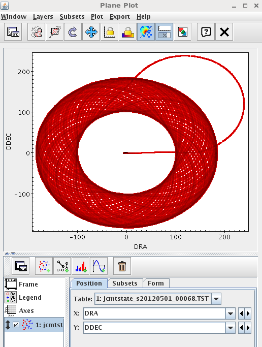
The scan pattern of a JCMT raw SCUBA-2 observation is being shown.

Worked Example

Take a reduced spectral cube, measure the noise on a blank part of the spectrum. Compare this noise with the measured noise from the Variance array.

First of all, we will open our cube in Gaia in order to identify a blank region of the spectra over which to measure the noise.

Finding a blank spectral section in Gaia.

The region from -265.0 to -78 km/s looks like it is very blank — we will use this to measure the noise.

You can either perform the collapse within Gaia by using the ‘collapse’ button on the Spectral cube window, and then either save the file or use the imaging tool in Gaia to examine the statistics, or you can use the command line. The command line is more repeatable.

First we will use KAPPA’s collapse command to collapse over the blank region. This command supports a wide range of estimators allowing you to produce integrated maps, RMS estiamtes and moment maps. Please see the documentation for full details. Here we will use the sigma estimator to get the standard deviation in that region.

collapse in=co32_cube.sdf axis=vrad low=-265.0 high=-78.0 estimator=sigma out=co32_noisemap.sdf

Note that we have to give the velocity range as floating points; if we give integers it will assume we mean pixel coordinates instead of km/s.

Now use the stats command to look at the values.

$ stats co32_noisemap.sdf 

   Pixel statistics for the NDF structure
/export/data/sgraves/sd/tutorial-data/JCMT_HETERODYNE_analysis_tutorial_2016/co
32_noisemap

      Title                     : Ros6
      NDF array analysed        : DATA

         Pixel sum              : 11429.2
         Pixel mean             : 0.829648
         Standard deviation     : 0.390908
         Skewness               : 2.14229
         Kurtosis               : 4.21748
         Minimum pixel value    : 0.518394
            At pixel            : (-12, -13)
            Co-ordinate         : (6:34:43.1, 4:11:20)
         Maximum pixel value    : 2.65666
            At pixel            : (60, -30)
            Co-ordinate         : (6:34:14.2, 4:09:38)
         Total number of pixels : 14042
         Number of pixels used  : 13776 (98.1%)
         No. of pixels excluded : 266 (1.9%)

Across the whole map we have a noise of 0.83+/-0.39 K

You can also open this map in Gaia, and use the Image Analysis->Image regions toolbar to measure the noise only in the center of the map.

gaiadisp co32_noisemap.sdf

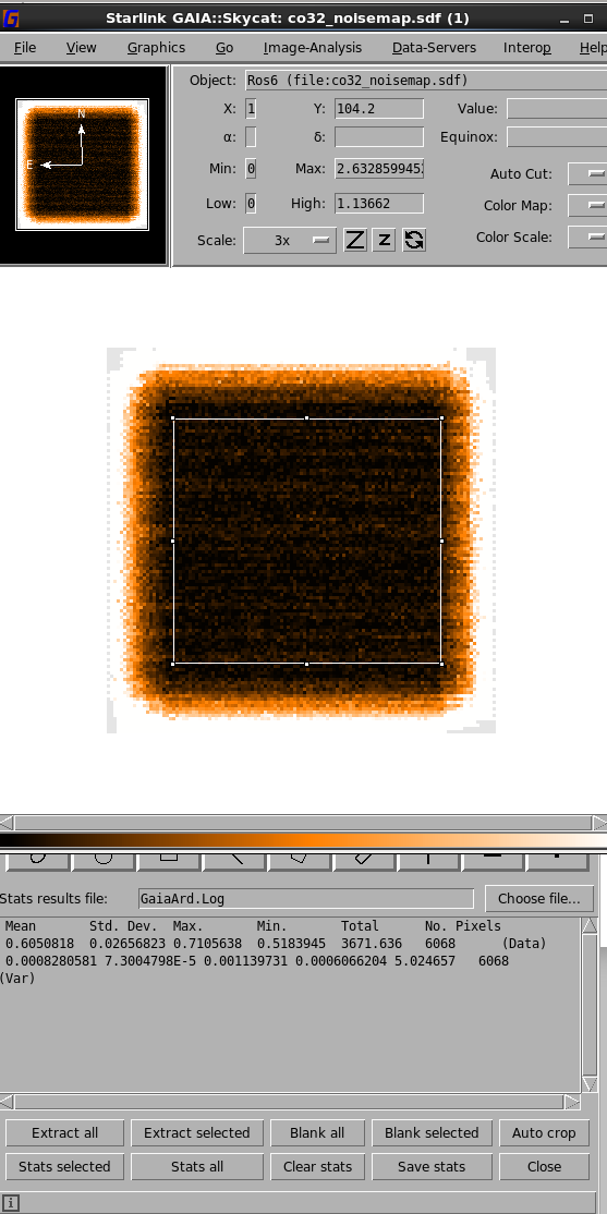
Using the Image Regions command to measure the average noise across the centre of a noise map.

Worked Example

We will use sqorst (SQuash OR STretch) to rebin the data onto 1.0 km/s channels. We will accept the default method of rebinning.

sqorst in=co32_cube.sdf axis=3 mode=pixelscale pixscale=1.0 out=co32_1kms.sdf method=auto

Now, we will repeat the previous collapse command on this file in order to measure the noise after rebinning. Because we set the collapse limits in terms of a velocity instead of using a pixel index, we don’t have to change them after rebinning.

collapse in=co32_1kms.sdf axis=vrad low=-265.15 high=-78.05 estimator=sigma out=co32_1kms_noisemap.sdf

As before, we see the results with stats:

$ stats co32_1kms_noisemap.sdf
    Pixel statistics for the NDF structure
/export/data/sgraves/sd/tutorial-data/JCMT_HETERODYNE_analysis_tutorial_2016/co
32_1kms_noisemap

      Title                     : Ros6
      NDF array analysed        : DATA

         Pixel sum              : 8072.22
         Pixel mean             : 0.585963
         Standard deviation     : 0.277194
         Skewness               : 2.13845
         Kurtosis               : 4.24379
         Minimum pixel value    : 0.341995
            At pixel            : (17, -12)
            Co-ordinate         : (6:34:31.5, 4:11:26)
         Maximum pixel value    : 1.91068
            At pixel            : (-19, -58)
            Co-ordinate         : (6:34:45.9, 4:06:50)
         Total number of pixels : 14042
         Number of pixels used  : 13776 (98.1%)
         No. of pixels excluded : 266 (1.9%)

Here you can see we now have a mean RMS noise in our regridded map of 0.59+/0.28 K. if you wish, you can verify that this has approximately followed the radiometer equation.

We can also compare the noise we have measured on the map with the noise in the VARIANCE component of the file. The easiest way is using the ‘comp’ option in stats to set which component to analyse (DATA is the default), and selecting the ERROR component, defined as the square root of the variance component.

$stats co32_1kms.sdf comp=ERROR


   Pixel statistics for the NDF structure
/export/data/sgraves/sd/tutorial-data/JCMT_HETERODYNE_analysis_tutorial_2016/co
32_1kms

      Title                     : Ros6
      NDF array analysed        : ERROR

         Pixel sum              : 6.0305e+06
         Pixel mean             : 0.550634
         Standard deviation     : 0.267865
         Skewness               : 2.21899
         Kurtosis               : -2.97147
         Minimum pixel value    : 0.364528
            At pixel            : (-37, 6, -397)
            Co-ordinate         : (6:34:53.1, 4:13:14, -380.4388)
         Maximum pixel value    : 1.63818
            At pixel            : (57, 51, -397)
            Co-ordinate         : (6:34:15.4, 4:17:44, -380.4388)
         Total number of pixels : 11163390
         Number of pixels used  : 10951920 (98.1%)
         No. of pixels excluded : 211470 (1.9%)

We see a noise from the variance component of 0.55 +/- 0.26 K, compared with 0.59 +/- 0.28 K measured across one part of the empty spectra. The variance component was generated by SMURF’s gridding command ‘makecube’, and be default is generated from the Tsys values of the input spectra.

Worked Example

We will use the SCUBA-2 map provided in the sample data, <code>scuba2_map.sdf</code>. This is the same as the <code>gs20120501_68_850_reduced.sdf</code> file provided in the SCUBA-2 tutorial <code>example_reduced</code> data directory

There are several ways you can do this. The simplest is to examine the ERROR component of the data.

$stats scuba2_map.sdf comp=ERROR

Pixel statistics for the NDF structure
/export/data/sgraves/sd/tutorial-data/JCMT_HETERODYNE_analysis_tutorial_2016/sc
uba2_map

      Title                     : G34.3
      NDF array analysed        : ERROR

         Pixel sum              : 1640087.30197531
         Pixel mean             : 41.0555547705848
         Standard deviation     : 50.659757537598
         Skewness               : 3.90590482923681
         Kurtosis               : 26.0299464638736
         Minimum pixel value    : 10.6386591437756
            At pixel            : (-3, 23, 1)
            Co-ordinate         : (18:53:19.667, 1:16:26.30, 0.00085)
         Maximum pixel value    : 1157.3041341558
            At pixel            : (-13, 122, 1)
            Co-ordinate         : (18:53:22.334, 1:23:02.30, 0.00085)
         Total number of pixels : 58081
         Number of pixels used  : 39948 (68.8%)
         No. of pixels excluded : 18133 (31.2%)

You can also see this in Gaia by going to Image Analysis-> Image Regions. Select the region you want to get statistics over and use the ‘Stats Selected’ button to generate the statistics. you can also use this to compare the noise in a blank part of the sky with the noise in the variance component.

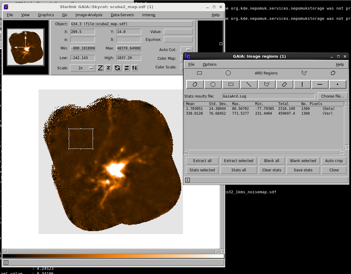
Measuring the noise in a blank field of a SCUBA-2 map with the Gaia Image Regions toolbar.

In the example shown in the screen shot above, the Std. Deviation of the data area is 24.4 (measuring the RMS noise in that region); by comparison the noise in the Variance array has a mean value in that region of 338, corresponding to an error of 18.4. Fairly close, but there is clearly some difference!

Another method, designed to be used on reductions of a single observation, is to run the PICARD recipe SCUBA2_MAPSTATS on your file. This would like so:

$ picard -log sf -nodisplay SCUBA2_MAPSTATS scuba2_map.sdf 
Picard Says: No display will be used
Picard Says: Pre-starting mandatory monoliths...Done
Checking for next data file: /export/data/sgraves/sd/tutorial-data/JCMT_HETERODYNE_analysis_tutorial_2016/scuba2_map.sdf
Storing: scuba2_map
Picard Says: Creating temporary bad observation rules file
A new group 20120501#-1 has been created
Overriding PICARD instrument class to PICARD_SCUBA2_850
Sorting Groups
REDUCING: scuba2_map
Using recipe SCUBA2_MAPSTATS specified on command-line
Processing data for G34.3

Calling _WRITE_MAPSTATS_LOGFILE_: write logfile with results from image analysis
Writing results to log.mapstats...
Cropping map using: RA= 18:53:18.6, Dec= 01:14:58.26, RADIUS=120.
RMS is 13.5415200736753

Recipe took 2.018 seconds to evaluate and execute.

Picard processing complete
Processed one recipe which completed successfully
Exiting...

In the output directory, you will now find a logfile anmed log.mapstats:

$cat log.mapstats
# Map results: noise, NEFD, exp_time log file - created on Thu Jan 25 20:45:30 2018 UT
#
# (YYYYMMDD.frac) (YYYY-MM-DDThh:mm:ss) () () () (um) (deg)  () ()  () () (s)  (s)  ()  ()  ()  ()  (")  (")  ()  ()  ()  ()  ()
# UT   HST  Obs  Source  Mode  Filter  El  Airmass  Trans  Tau225  Tau  t_elapsed  t_exp  rms  rms_units  nefd  nefd_units  RA  Dec  mapsize  pixscale  project  recipe  filename
20120501.6984144  2012-05-01T06:45:43    68  G34.3  daisy        850  52  1.26  0.783  0.047  0.194  318  68.08  1.354E+01  mJy/bm  1.078E+02  mJy.s^0.5   18:53:18.6   01:14:58.26  240.0  4.0  M12AEC05  REDUCE_SCAN  scuba2_map

This summarises information about the observation, as well as calculating the noise over central portion of the MAP, and the NEFD (Noise Equivalent Flux Density, usually used for tracking instrumental performance). If you run this command on a coadded map, it cannot accurately fill in most of the columns about the observation.

Worked Example

By default, the X: and Y: boxes in Gaia will show you the pixels relative to the bottom left of the map. Normally, the NDF PIXEL coordinates (relative to the pixel origin shown in ndftrace) are more useful. You can see these values in Gaia in two ways: one, you can open Image Analysis->Change Coordinates-> Show All Coordinates. This will bring up a seperate window that will show you the PIXEl (as well as GRID, AXIS< FRACTION and SKY) coordinates of your cursor as you move it around in the Gaia window.

Alternatively, you can start Gaia with the -pixel_indices=1 flag, and it will then show you the NDF PIXEL coordinates by default.

gaia -pixel_indices 1 scuba2_map.sdf

When you need to identify the pixel ranges, you can then use these coordinates. Test this out by finding the pixel values for a section of the map, then use ndfcopy and an NDF section to copy that part out. Open your new map in Gaia and verify you copied the part you were looking for. Remember that pixel indices have to be given in integers!

ndfcopy scuba2_map.sdf\(10:65,-5:53\) extracted.sdf
gaia -pixel_indices 1 extracted.sdf &

Worked Example

The main difficulity with this is formatting the strings correctly and using shell escapes. D There are several ways this could be done. One example is

ndfcopy scuba2_map.sdf\(18h53m16.3s:18h53m01.4s,1d14m35s:1d18m27.6s\) extracted2.sdf

In this example, don’t include any spaces next to the comma in the centre of the NDF section or it won’t be parsed correctly. If instead of using backslashes for your shell escapes you enclose the entire NDF and NDF section inside double and single quotes, then you can use spaces after the comman. E.g.:

ndftrace "'scuba2_map.sdf(18h53m16.3s:18h53m01.4s, 1d14m35s:1d18m27.6s)'"

NDF sections can be passed to commands anywhere an entire NDF could be passed. Once you get the hang of them they are a very useful feature of Starlink.

Worked Example

You can do this using the PICARD task CROP_SCUBA2_IMAGES:

$ picard -log sf CROP_SCUBA2_IMAGES scuba2_map.sdf 
Setting up display infrastructure (display tools will not be started until necessary)...Done
Picard Says: Pre-starting mandatory monoliths...Done
Checking for next data file: /export/data/sgraves/sd/tutorial-data/Starlink_Analysis/scuba2_map.sdf
Storing: scuba2_map
A new group 20120501#-1 has been created
Overriding PICARD instrument class to PICARD_SCUBA2_850
Sorting Groups
REDUCING: scuba2_map
Using recipe CROP_SCUBA2_IMAGES specified on command-line
Processing data for G34.3

Calling _CROP_SCUBA2_IMAGE_: trim image to specified map size
Trimming image to specified map size
Trimming scuba2_map...
Cropping map using: RA= 18:53:18.6, Dec= 01:14:58.26, RADIUS=120.
Removing temporary files...
Checking scuba2_map_crop...	Keeping extension
Recipe took 1.308 seconds to evaluate and execute.

Picard processing complete
Processed one recipe which completed successfully
Exiting...

Picard Says: Goodbye

By default this will use the center position of the original observation, and the ‘radius’ of the central area of the SCAN type, and produce a square cut out around the center.

If you wish to crop out a circular area or a larger area, you can provide a recpars file to alter this. E.g. to crop out a CIRCLE of radius 250″, you would save in a text file:

[CROP_SCUBA2_IMAGES]
CROP_METHOD=CIRCLE
MAP_RADIUS=250

Save this file as e.g. recpars.txt and then run

$ picard -log sf CROP_SCUBA2_IMAGES -recpars=recpars.txt scuba2_map.sdf 
Setting up display infrastructure (display tools will not be started until necessary)...Done
Picard Says: Pre-starting mandatory monoliths...Done
Checking for next data file: /export/data/sgraves/sd/tutorial-data/Starlink_Analysis/scuba2_map.sdf
Storing: scuba2_map
A new group 20120501#-1 has been created
Overriding PICARD instrument class to PICARD_SCUBA2_850
Sorting Groups
REDUCING: scuba2_map
Using recipe CROP_SCUBA2_IMAGES specified on command-line
Processing data for G34.3

Calling _CROP_SCUBA2_IMAGE_: trim image to specified map size
Trimming image to specified map size
Output image will be a circle of radius 250 arcsec
Masking the weights and exposure time images...
Removing temporary files...
Checking scuba2_map_tmpmask...	Removing
Checking scuba2_map_crop...	Keeping extension
Recipe took 2.668 seconds to evaluate and execute.

Picard processing complete
Processed one recipe which completed successfully
Exiting...

Picard Says: Goodbye

ARD format files are fairly straight forward, so they can be made yourself. A simple file to extract out a ring of inner radius 70″, outer radius 100″ and centered on RA=18:53:18.7, Dec=1:14:54.3 would be:

COFRAME(SKY, SYSTEM=FK5, equinox=2000)
CIRCLE(18:53:18.7,1:14:54.3, :1:40.) .AND. .NOT. CIRCLE(18:53:18.7,1:14:54.3, :1:10.0)

Note that we define the radii in(third element of the CIRCLE command) in degrees:arcminutes:arcseconds. To create an annulus we have defined one larger circle, and then said to exclude the central region of the circle.

We save this as e.g. file ARD_ring.ard, and then we can apply it with ardmask.

ardmask in=scuba2_map.sdf ardfile=ARD_ring.ard out=scuba2_map_2d.sdf inside=False

Note that we need to remove the redundant third axis of the data — here we do this with ndf copy.

ndfcopy in=scuba2_map.sdf out=scuba2_map2d.sdf trim=true trimwcs=true 

The result should look like:

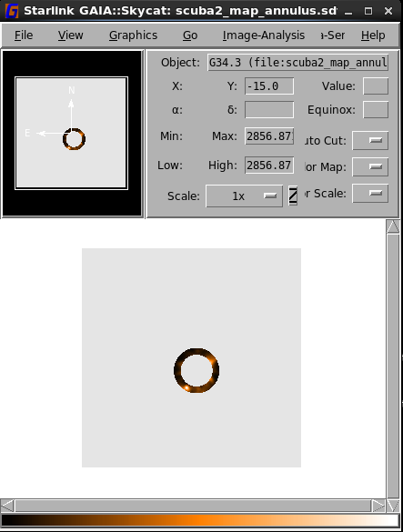
An annulus created with an ARD file.

You could also try using the ARDGEN interactive utility to create an ARD file. First of all, you need to display the image in an Xwindow using the KAPPA’s display command:

display scuba2_map.sdf dev=xw mode=faint

(This displays the map in the xwindows graphics device, using mode=faint so that you are not prompted to give a low and high value to scale between.)

You then run the command ardgen dev=xw and follow the prompts, selecting the shape you want to make and clicking in the xwindow to mark shapes. Remember you can use the ? at a command line prompt to see the help.

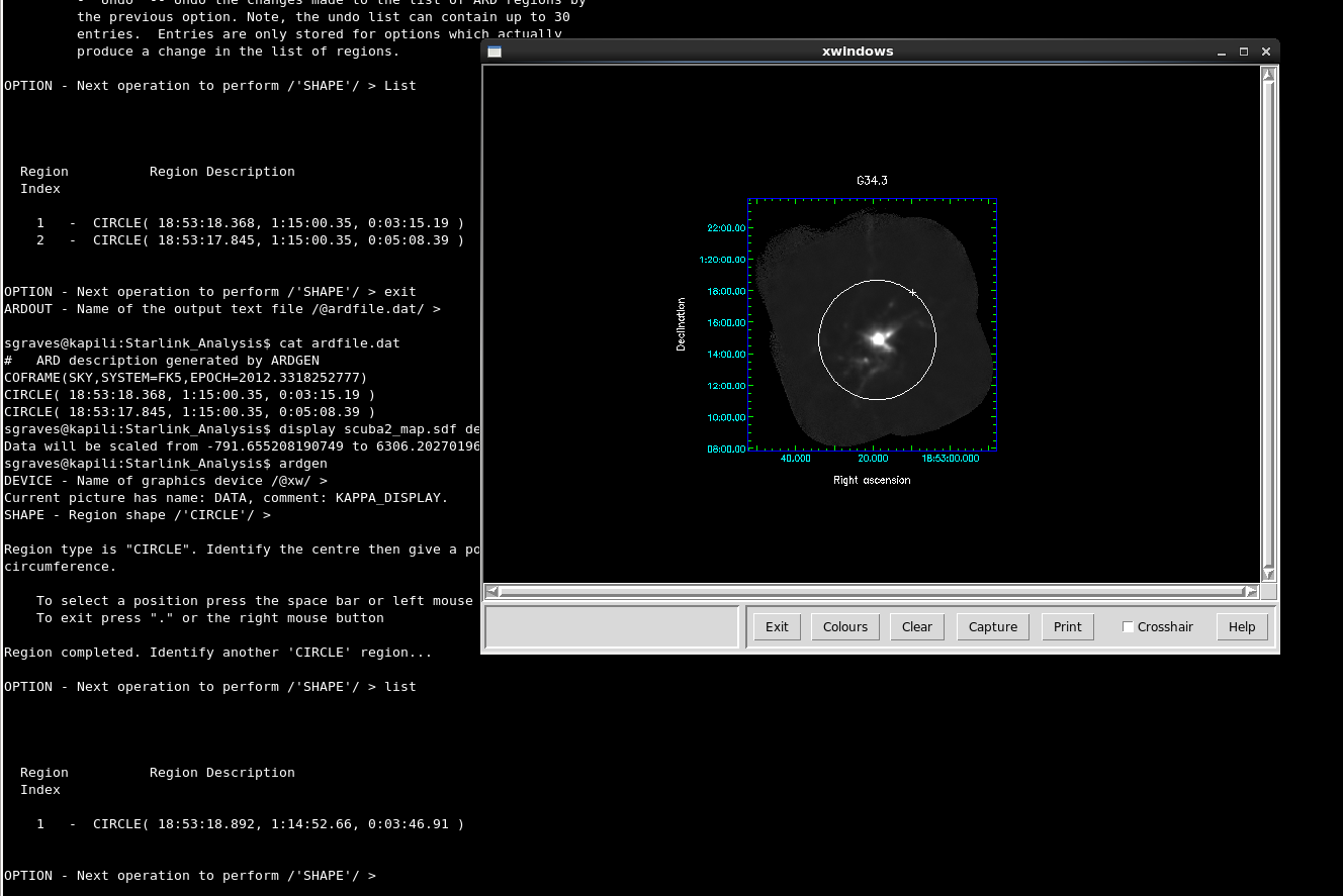
ARDGEN in use. you can see the circular shape defined by the user overlain on the image shown with display.

Mask out all pixels in a cube or map with a detection of less than 5 sigma (try errclip)

The command errclip can be used to clip a map or cube based on SNR levels, using the variance component of the map to define the snr. You can use it like:

errclip in=co32_cube.sdf mode=SNR out=co32_clipped5sigma limit=5.0

Open the resulting map in Gaia and take a look at it: you’ll see that the baseline and linewing regions are marked as bad, and only the strong parts of the line centre in bright regions are remaining.

Mask out all spectra in a cube where the peak of the spectra has a detection of less than 5 sigma. Try using makesnr, thresh, manic and copybad.

Often, its useful not to clip out individual channels on the basis of the noise limit, but instead to clip out only whole spectra where the peak was not detected at greater than 5 sigma.

First of all, we will need to collapse the cube down to a map of the peak values in each spectrum, using collapse. You can determine the velocity range to perform the collapse over by inspecting the cube in Gaia.

collapse in=co32_cube.sdf axis=vrad low=-6.5 high=25.67 estimator=max out=maxvalue

(If you would prefer to clip based on a detection in the integrated line, you could use the estimator=integ option instead.)

We will now create an SNR map from this 2-D peak map with the makesnr command:

makesnr in=maxvalue.sdf out=snr.sdf minvar=0.0

Then we use the thresh command to set bad all pixels with an SNR less than 5. We also select a spurious high value to set bad, as we have to provide both thrlo and thrhi options; this won’t cause any problems.

thresh in=snr out=snr_thr5 thrlo=5.0 thrhi=5000 newlo=bad newhi=bad

You now need to grow this mask into a 3-D mask you can apply to your original map. To do this we first need to find out what the pixel indices of are input cube are;

$ ndftrace co32_cube.sdf 

   NDF structure
/export/data/sgraves/sd/tutorial-data/Starlink_Analysis/co32_cube:
      Title:  Ros6
      Label:  TA*   corrected antenna temperature
      Units:  K

   Shape:
      No. of dimensions:  3
      Dimension size(s):  119 x 118 x 1880
      Pixel bounds     :  -57:61, -58:59, -940:939
      Total pixels     :  26398960

   Data Component:
      Type        :  _REAL
      Storage form:  SIMPLE
      Bad pixels may be present

   Variance Component:
      Type        :  _REAL
      Storage form:  SIMPLE
      Bad pixels may be present

   World Co-ordinate Systems:
      Number of co-ordinate Frames: 5

      Current co-ordinate Frame (Frame 5):

        Frame title         : "3-d compound coordinate system"
        Domain              : SKY-DSBSPECTRUM
        First pixel centre  : 6:35:01.2, 4:06:50, -381.1352

           Axis 1:
              Label              : Right ascension
              Units              : hh:mm:ss.s
              Nominal Pixel scale: 5.99999 arc-sec

           Axis 2:
              Label              : Declination
              Units              : ddd:mm:ss
              Nominal Pixel scale: 5.99999 arc-sec

           Axis 3:
              Label              : Radio velocity (USB)
              Units              : km/s
              Nominal Pixel scale: 0.4233065 km/s


   Extensions:
      FITS             
      SMURF            
      PROVENANCE       


   History Component:
      Created    :  2014 Nov 20 09:22:05
      No. records:  22
      Last update:  2018 Jan 25 22:26:20 (WCSATTRIB       (KAPPA 2.5-5))
      Update mode:  NORMAL

We can see here that our c32_cube goes from -940:939 in pixels in the 3rd, velocity, axis. We will now use the command manic to grow our 2D mask into a 3D mask we can apply to our original data; manic increases the dimensionality of the cube by (in this case) repeating the image plane pixels in every plane we add in the third dimension. The command we use is:

manic in=snr_thr5 out=cube_mask axes=\[1,2,0\] ubound=939 lbound=-940

Finally, we copy the bad pixel mask from this cube to our original CO 3-2 cube, and then open the masked map in Gaia to examine it.

copybad in=co32_cube.sdf ref=cube_mask.sdf  out=co32_masked.sdf
gaiadisp co32_masked.sdf

Extracting Values

You can always of course use the stats command to get the sum/mean etc value for small regions, or within extracted NDF sections or ARD masked/extracted areas, and you may find that sufficient for reading out some of your values. The pluck command can be used to easily get data values at a specific point on the map however, or to extract the whole spectra from that point.

You can use pluck interactively, but here we will use it by giving it a text file. The format of the input catalogue is:

6:34:37.7 4:12:37.20 1
6:34:32.77 4:13:09.77 1
6:34:24.47 4:08:56.91 1

Note that you have to provide a value for axis 3, even though the output will include all values from that axis. We then run the command with:

$ pluck in=co32_cube.sdf axes=vrad mode=file coin=spectra_positions.txt container=True out=container_spectra.sdf method=linear
Creating
/export/data/sgraves/sd/tutorial-data/Starlink_Analysis/container_spectra.PLUCK
_1.
Creating
/export/data/sgraves/sd/tutorial-data/Starlink_Analysis/container_spectra.PLUCK
_2.
Creating
/export/data/sgraves/sd/tutorial-data/Starlink_Analysis/container_spectra.PLUCK
_3.

We used a linear resampling method to extract the pixels; others are available, but may require setting the params paramter to use. See the documentation for details. We now have an output file container_spectra.sdf which contains 3 input spectra as separate NDFs. We can copy them out to their own files with:

ndfcopy container_spectra.PLUCK_1 pluck_1
ndfcopy container_spectra.PLUCK_2 pluck_2
ndfcopy container_spectra.PLUCK_3 pluck_3

If you use ndftrace to look at one of the spectra, it includes all the information about the spatial position it was extracted from.

$ ndftrace pluck_*.sdf 

   NDF structure
/export/data/sgraves/sd/tutorial-data/Starlink_Analysis/pluck_1:
      Title:  Ros6
      Label:  TA*   corrected antenna temperature
      Units:  K

   Shape:
      No. of dimensions:  3
      Dimension size(s):  1 x 1 x 1880
      Pixel bounds     :  1:1, 1:1, -940:939
      Total pixels     :  1880

   Data Component:
      Type        :  _REAL
      Storage form:  SIMPLE
      There are no bad pixels present

   Variance Component:
      Type        :  _REAL
      Storage form:  SIMPLE
      There are no bad pixels present

   World Co-ordinate Systems:
      Number of co-ordinate Frames: 5

      Current co-ordinate Frame (Frame 5):

        Frame title         : "3-d compound coordinate system"
        Domain              : SKY-DSBSPECTRUM
        First pixel centre  : 6:34:37.7, 4:12:37, -381.1352

           Axis 1:
              Label              : Right ascension
              Units              : hh:mm:ss.s
              Nominal Pixel scale: 6.00000 arc-sec

           Axis 2:
              Label              : Declination
              Units              : ddd:mm:ss
              Nominal Pixel scale: 6.00000 arc-sec

           Axis 3:
              Label              : Radio velocity (USB)
              Units              : km/s
              Nominal Pixel scale: 0.4233065 km/s


   Extensions:
      FITS             
      SMURF            
      PROVENANCE       


   History Component:
      Created    :  2014 Nov 20 09:22:05
      No. records:  24
      Last update:  2018 Jan 26 02:41:53 (NDFCOPY         (KAPPA 2.5-5))
      Update mode:  NORMAL

You can also view the spectra in splat with:

splat pluck_*.sdf&

Or display them with KAPPA’s linplot command:

linplot pluck_1 dev=xw

Worked Example

Setting a new coordinate system in a map is easy. However, please note that this will not change the pixels in anyway: if you want to regrid your map onto a pixel grid aligned with a new coordinate system (this can matter more for extremely large maps), then you should look into the regrid command. Starlink NDF files, unlike FITS files, generally have multiple WCS systems associated with them, with defined transformations between them. Therefore, changing the coordinates only involves running wcsattrib to tell it to set the current system to your desired one. In this case, you will do:

wcsattrib ndf=co32_cube.sdf mode=set name=System newval=Galactic

And thats it!

You can verify it by opening and Gaia and seeing which coordinate system is the default, or by converting to a FITS file with:

convert
ndf2fits co32_cube.sdf co32_galactic.fits

and opening it with your favourite non Gaia program. For example, see what the Python plotting program APLpy made of the FITS version of this file:

I highly recommend reading the documentation for fit1D: it has a lot of options, but is very powerful. As a quick overview, here is one example of using it.

First, create a configuration file. An example one can be found in $STARLINK_DIR/bin/smurf/smurf_fit1d.def , including descriptions of various parameters. We are going to use the basic paramters, and only provide updated values for the range parameter. This determines the radio velocity range we will fit the profiles within, and we will use -12 to 88 km/s.

This mostly-default config will fit a single Gausshermite2 to each spectrum. We define our config file as:

^$SMURF_DIR/smurf_fit1d.def
range=(-12.0,88.0)

We save it as myfit1d.def, and then run our command as:

$ fit1d in=co32_masked.sdf out=fittedprofiles.sdf rms=! config=^myfit1d.def
Copying input file 1 to output for fitting...
Fitting data using 1 GAUSSHERMITE2(s) over pixel range [873,1109]
...Will use 16 threads to fit 14042 profiles.
(FitProfileThread 16) ...at profile 14000 - 845 of 887 (i=26318120)
...Writing parameter cubes and finishing up.

(A Caret, ^, indicates to read the contents of the text file that follows.)

If you open the resulting cube up in Gaia, and also open the original map in Gaia next to it via the File->new Window option, you can use the Open Cube->Options->Slave to move about in one cube and see spectra from both cubes. Alternatively, you can use the sub command to view the residuals from the fit.

sub in1=co32_masked.sdf in2=fittedprofiles.sdf out=residuals.sdf

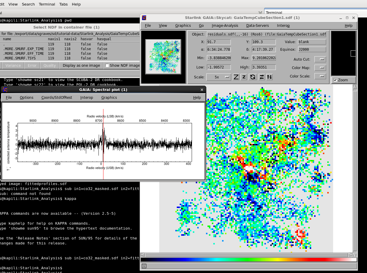
Examining the residuals from a fit1d line fitting procedure with Gaia.

If you’re not familiar with Fellwalker, you should read the description of the algorithm in the CUPID manual, or David Berry’s 2015 A&C paper.

We first of all need to select our configuration parameters. Here, we are going to look for all clumps of 5 sigma above the noise, and we will subdivide neighbouring clumps into separate clumps if they have gaps between their peaks of at least 3sigma. We will follow the clumps down to 3 sigma above the noise. The config file we need to define is then:

FellWalker.Noise=3*RMS
FellWalker.MinHeight=5*RMS
FellWalker.MinDip=3*RMS

We save that into a text file, here named config.lis, and then we can call findclumps (after initialising cupid) as:

findclumps scuba2_map.sdf out=scuba2_clumps.sdf \
      outcat=clumpcat.FITS method=fellwalker deconv=no accept

We have to provide the special keyword accept indicating that all other parameters that would be prompted for should use their default value. This is necessary if you don’t want to be prompted to accept the default RMS value (calculated from the VARIANCE array);
findclumps will otherwise wait for you to either accept the calculated RMS or give a different value.

We now have an output catalog in clumpcat.FITS that we can open and view with Topcat, and an output clumpmask in scuba2_clumps.sdf that we can view in Gaia. Go ahead and open the mask in Gaia:

gaia scuba2_clumps.sdf&

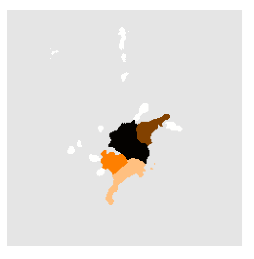
Example of a clump mask (the output from findclumps)

You can see the output is a mask over the full area of each clump, where the value of that clump is the same as the clump index in the output catalogue. Pixels not assigned to a clump are set as BAD values.

The output file also has a special CUPID extension; for fellwalker, this contains an array of all the identified clumps with the data values from the original data included. You can access these like you do any other NDF extension, so to copy out (for example) clump 3 to its own NDF file you would do:

ndfcopy scuba2_clumps.sdf.more.CUPID.CLUMPS\(3\) clump3.sdf

Or you can even open that clump directly in Gaia with:

gaiadisp scuba2_clumps.sdf.more.CUPID.CLUMPS\(3\)

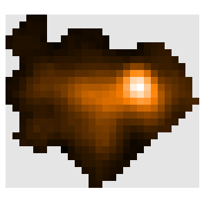
The 3rd Clump found by Fellwalker, as saved in the CUPID.CLUMPS extension.